Volterra System Identification on Electric Drives
This example shows how to identify a nonlinear dynamical system using CPKM (CP Tensor-Network Kernel Machine) with a polynomial Volterra feature map.
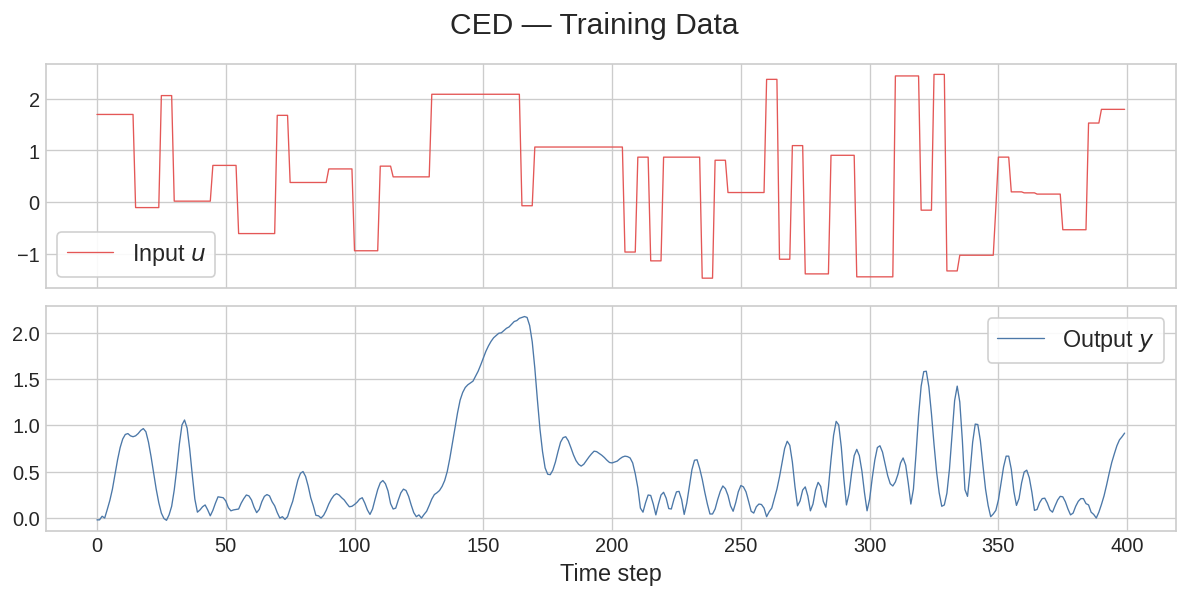
We use the Coupled Electric Drives (CED) benchmark dataset — a standard SISO nonlinear benchmark from the sysid community.
What you will learn:
- How to cast SISO nonlinear sysid as supervised regression
- How to build a Volterra feature map with
VoltFeature - How to train a
CPKMmodel with ALS on time-series data
import jax
import numpy as np
import jax.numpy as jnp
import matplotlib as mpl
import matplotlib.pyplot as plt
import nonlinear_benchmarks as nb
from sklearn.preprocessing import MinMaxScaler

from tnkm.models import CPKM
from tnkm.optim import train_als
from tnkm.features import ProductFeatures, VoltFeature

jax.config.update("jax_enable_x64", True)
plt.style.use("seaborn-v0_8-whitegrid")

RC_PARAMS = {
    'figure.facecolor': 'white',
    'font.size': 10,
    'axes.labelsize': 14,
    'axes.grid': True,
    'lines.linestyle': '-',
    'legend.fontsize': 14,
    'xtick.labelsize': 12,
    'ytick.labelsize': 12,
    'axes.titlesize': 16,
    'figure.max_open_warning': 50,
    "legend.frameon": True,
    "legend.framealpha": 0.9,
}

COLORS = dict(
    blue2="#4C78A8",
    red2="#E45756",
    green2="#71b553",
    purple2="#af4d7d"
)
Load & Explore Data
The CED benchmark provides two training sets and two test sets. We use the first of each.
Note
Unlike the ML examples, we do not shuffle the data. The temporal ordering of samples is essential for time-series models.
We apply MinMaxScaler to the raw input signal and output using training
statistics only.
train_sets, test_sets = nb.CED()
u_train, y_train = train_sets[0]
test_1, _ = test_sets
u_test, y_test = test_1.u, test_1.y

print(f"Train: {len(u_train)} samples")
print(f"Test: {len(u_test)} samples")

# MinMax normalization using training statistics
x_scaler, y_scaler = MinMaxScaler(), MinMaxScaler()
X_tr_sc = jnp.array(x_scaler.fit_transform(np.array(u_train)[:, None]))
y_tr_sc = jnp.array(
    y_scaler.fit_transform(np.array(y_train).reshape(-1, 1)).squeeze()
)

with mpl.rc_context(RC_PARAMS):
    fig, axes = plt.subplots(2, 1, figsize=(10, 5), sharex=True)
    axes[0].plot(u_train, color=COLORS['red2'],  lw=0.8, label="Input $u$")
    axes[1].plot(y_train, color=COLORS['blue2'], lw=0.8, label="Output $y$")
    for ax in axes:
        ax.legend()
    axes[1].set_xlabel("Time step")
    plt.suptitle("CED — Training Data", fontsize=18)
    plt.tight_layout()
    plt.show()
Train: 400 samples
Test: 100 samples
Build & Train CPKM
A Volterra model predicts the current output from a window of past inputs:
VoltFeature(m_order) builds this feature vector internally.
Using d_dim=volt_order copies in ProductFeatures creates a
degree-volt_order Volterra kernel — the tensor product captures
nonlinear cross-lag interactions up to the specified order.
| Parameter | Role |
|---|---|
m_order |
Memory length — number of past input samples used |
volt_order |
Volterra kernel order — degree of nonlinearity |
rank |
CP rank — number of rank-1 terms in the Volterra kernel |
ALS updates one CP core at a time while keeping the others fixed.
gamma_w controls L2 regularization.
m_order = 10 # memory length
volt_order = 3 # Volterra kernel order (degree of nonlinearity)
rank = 10 # CP rank

features = ProductFeatures(
    VoltFeature(m_order, p_input=1),
    d_dim=volt_order
)
model = CPKM(features, rank=rank, seed=0)

train_als(model, X_tr_sc, y_tr_sc, n_epoch=10, gamma_w=1e-1, beta_e=1.0)

# One-step-ahead on train
y_tr_pred_sc = model.predict(X_tr_sc)
y_tr_pred = y_scaler.inverse_transform(
    np.array(y_tr_pred_sc).reshape(-1, 1)).squeeze()
y_tr_orig = y_scaler.inverse_transform(
    np.array(y_tr_sc).reshape(-1, 1)).squeeze()

# Build and normalize test features
X_te_sc = jnp.array(x_scaler.transform(np.array(u_test)[:, None]))
y_te_sc = jnp.array(
    y_scaler.transform(np.array(y_test).reshape(-1, 1)).squeeze()
)
y_te_pred_sc = model.predict(X_te_sc)
y_te_pred = y_scaler.inverse_transform(
    np.array(y_te_pred_sc).reshape(-1, 1)).squeeze()
y_te_orig = y_scaler.inverse_transform(
    np.array(y_te_sc).reshape(-1, 1)).squeeze()

rmse_tr = np.sqrt(np.mean((y_tr_orig - y_tr_pred) ** 2))
rmse_te = np.sqrt(np.mean((y_te_orig - y_te_pred) ** 2))
print(f"Train RMSE (one-step): {rmse_tr:.4f}")
print(f"Test RMSE (one-step): {rmse_te:.4f}")
Train RMSE (one-step): 0.2188
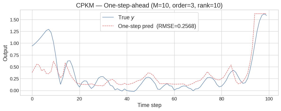
Test RMSE (one-step): 0.2568
One-step-ahead Prediction
In one-step-ahead prediction the model sees the true past inputs at every step. This is the easiest regime — it shows whether the model has learned the input-output mapping, but does not test closed-loop stability.
with mpl.rc_context(RC_PARAMS):
    fig, ax = plt.subplots(figsize=(10, 4))
    ax.plot(y_te_orig, color=COLORS['blue2'], lw=1.0, label="True $y$")
    ax.plot(y_te_pred, color=COLORS['red2'],  lw=1.0,
        label=f"One-step pred  (RMSE={rmse_te:.4f})", linestyle="--"
    )
    ax.set_xlabel("Time step")
    ax.set_ylabel("Output")
    ax.set_title(
        f"CPKM — One-step-ahead (M={m_order}, order={volt_order}, rank={rank})"
    )
    ax.legend()
    plt.tight_layout()
    plt.show()
Next Steps
- Add output feedback (NARX): use
build_lagged_datawith bothinput_lagsandoutput_lagsto include past output values in the regressor — this turns the model into a NARX (Nonlinear AutoRegressive with eXogenous input). The companionbuild_lagged_featurefunction can then be used withsimulate_recursivefor closed-loop simulation - Switch to TTKM: replace
CPKMwithTTKMfor potentially better compression at higher memory lengths - Increase Volterra order: increase
volt_order(e.g. 4 or 5) to capture higher-degree nonlinearities at the cost of more computation - Use both training sets: concatenate
train_sets[0]andtrain_sets[1]for more training data