Gaussian Kernel Regression on Airfoil Self-Noise
This example shows how to use TTKM (TT Tensor-Network Kernel Machine) with squared-exponential (Gaussian kernel) features and gradient-based training for multi-dimensional regression.
We use the Airfoil Self-Noise dataset (UCI) — 5 continuous inputs describing aerodynamic conditions, 1503 samples, target is scaled sound pressure level in dB.
What you will learn:
- How to build a
ProductFeaturesmap with per-dimensionSquaredExpFeature - How to train a
TTKMmodel withtrain_gradand an Optax optimizer - How different optimizers (SGD, Adam, Adan, Lion) affect convergence speed
import jax
import optax
import numpy as np
import jax.numpy as jnp
import matplotlib as mpl
import matplotlib.pyplot as plt
from ucimlrepo import fetch_ucirepo

from tnkm.models import TTKM
from tnkm.optim import train_grad
from tnkm.dataloader import DataLoader
from tnkm.features import ProductFeatures, SquaredExpFeature

jax.config.update("jax_enable_x64", True)
plt.style.use("seaborn-v0_8-whitegrid")

RC_PARAMS = {
    'figure.facecolor': 'white',
    'font.size': 10,
    'axes.labelsize': 14,
    'axes.grid': True,
    'lines.linestyle': '-',
    'legend.fontsize': 14,
    'xtick.labelsize': 12,
    'ytick.labelsize': 12,
    'axes.titlesize': 16,
    'figure.max_open_warning': 50,
    "legend.frameon": True,
    "legend.framealpha": 0.9,
}

COLORS = dict(
    blue2="#4C78A8",
    red2="#E45756",
    green2="#71b553",
    purple2="#af4d7d"
)
Load & Preprocess
The dataset has 5 continuous features (frequency, angle of attack, chord length, free-stream velocity, displacement thickness) and 1503 samples.
We apply:
- 80/20 train/test split with a fixed random seed for reproducibility
- Normalization of inputs to \([-1, 1]\) —
SquaredExpFeatureis defined on the Hilbert-space domain \([-v_\text{bound},\, v_\text{bound}]\), so we setv_boundlarger than the input range (herev_bound=3) - Standardization of the output (zero mean, unit variance)
Note
All statistics are computed on the training set only to avoid data leakage.
airfoil = fetch_ucirepo(id=291)
X_raw = airfoil.data.features.to_numpy().astype(float)
y_raw = airfoil.data.targets.to_numpy().squeeze().astype(float)

d_dim = X_raw.shape[1]

# 80/20 split
rng = np.random.default_rng(42)
idx = rng.permutation(len(X_raw))
n_train = int(0.8 * len(X_raw))
tr, te = idx[:n_train], idx[n_train:]
X_tr, X_te = X_raw[tr], X_raw[te]
y_tr, y_te = y_raw[tr], y_raw[te]

# Normalize inputs to [-1, 1] using training statistics
eps = 1e-8
x_min, x_max = X_tr.min(0), X_tr.max(0)
X_tr = 2 * (X_tr - x_min) / (x_max - x_min + eps) - 1
X_te = 2 * (X_te - x_min) / (x_max - x_min + eps) - 1

# Standardize output using training statistics
y_mean, y_std = y_tr.mean(), y_tr.std()
y_tr = (y_tr - y_mean) / (y_std + eps)
y_te = (y_te - y_mean) / (y_std + eps)

x_train, y_train, x_test, y_test = map(
    jnp.array, [X_tr, y_tr, X_te, y_te]
)

print(f"Train: {x_train.shape}, Test: {x_test.shape}, d_dim={d_dim}")
Train: (1202, 5), Test: (301, 5), d_dim=5
Build & Train TTKM
A TTKM model is defined by:
ProductFeatures— a per-dimension feature map. Here each dimension getsSquaredExpFeature(m_order, scale, v_bound, k_col=i), which approximates the Gaussian kernel via sinusoidal Hilbert-space basis functions.rank— the TT rank. Higher rank → more expressive model.
Key SquaredExpFeature parameters:
| Parameter | Role |
|---|---|
m_order |
Number of basis functions per dimension |
scale |
Length-scale: smaller → short-range, larger → smooth |
v_bound |
Domain half-width; set larger than the input range to avoid boundary effects |
Training uses train_grad, which requires three ingredients:
- A
DataLoader— wraps(x_train, y_train)into mini-batches - A loss function — built via
model.make_loss() - An Optax solver — e.g.
optax.adam
m_order = 8 # basis functions per dimension
scale = 0.1 # length-scale
v_bound = 3 # domain [-3, 3] ⊃ input range [-1, 1], avoids boundary effects
rank = 5 # TT rank
n_epoch = 100

features = ProductFeatures(
    [
        SquaredExpFeature(m_order, scale=scale, v_bound=v_bound, k_col=i)
        for i in range(d_dim)
    ]
)
model = TTKM(features, rank=rank, seed=0)

train_loader = DataLoader(x_train, y_train, batch_size=32, shuffle=True, seed=0)
loss_f = model.make_loss(gamma_w=1e-3, beta_e=1.0, reg_mode="cores")
solver = optax.adam(learning_rate=2e-2)

losses = train_grad(model, train_loader, solver, n_epoch=n_epoch, loss_f=loss_f)

y_train_pred = model.predict(x_train)
y_test_pred = model.predict(x_test)

train_mse = float(jnp.mean((y_train_pred - y_train) ** 2))
test_mse = float(jnp.mean((y_test_pred - y_test) ** 2))
print(f"Train MSE: {train_mse:.4f}")
print(f"Test MSE: {test_mse:.4f}")
Train MSE: 0.1336
Test MSE: 0.1829
Results
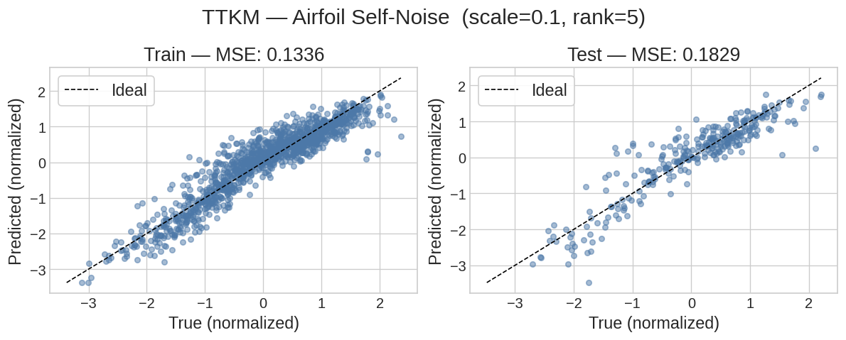
The two panels show predicted vs. actual sound pressure level (normalized) on train and test sets. Each point is one sample; the dashed line is the ideal \(\hat{y} = y\) reference. Points tight to the diagonal indicate accurate predictions.
A large train–test gap signals overfitting — try increasing gamma_w,
reducing rank, or increasing scale for a smoother prior.
with mpl.rc_context(RC_PARAMS):
    fig, axes = plt.subplots(1, 2, figsize=(10, 4))
    for ax, (y_true, y_pred, split) in zip(
        axes,
        [(y_train, y_train_pred, "Train"), (y_test, y_test_pred, "Test")],
    ):
        lo = min(float(y_true.min()), float(y_pred.min()))
        hi = max(float(y_true.max()), float(y_pred.max()))
        mse = float(jnp.mean((y_pred - y_true) ** 2))
        ax.scatter(y_true, y_pred, s=20, alpha=0.5, color=COLORS['blue2'])
        ax.plot([lo, hi], [lo, hi], "k--", lw=1, label="Ideal")
        ax.set_xlabel("True (normalized)")
        ax.set_ylabel("Predicted (normalized)")
        ax.set_title(f"{split} — MSE: {mse:.4f}")
        ax.legend()

    plt.suptitle(
        f"TTKM — Airfoil Self-Noise  (scale={scale}, rank={rank})",
        fontsize=18,
    )
    plt.tight_layout()
    plt.show()
Optimizer Comparison
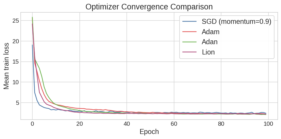
train_grad accepts any Optax optimizer, making it easy to swap solvers.
Here we compare four common choices — SGD with momentum, Adam, Adan, and Lion —
trained from the same initialization on the same data.
The plot shows the mean training loss per epoch for each optimizer.
solvers = {
    "SGD (momentum=0.9)": optax.sgd(learning_rate=1e-2, momentum=0.9),
    "Adam": optax.adam(learning_rate=1e-2),
    "Adan": optax.adan(learning_rate=1e-2),
    "Lion": optax.lion(learning_rate=1e-2),
}
color_keys = ["blue2", "red2", "green2", "purple2"]

all_losses = {}
for name, solver in solvers.items():
    mdl = TTKM(features, rank=rank, seed=0)
    loader = DataLoader(x_train, y_train, batch_size=32, shuffle=True, seed=0)
    lf = mdl.make_loss(gamma_w=1e-3, beta_e=1.0, reg_mode="cores")
    all_losses[name] = train_grad(mdl, loader, solver, n_epoch=n_epoch, loss_f=lf)

with mpl.rc_context(RC_PARAMS):
    fig, ax = plt.subplots(figsize=(8, 4))
    for (name, loss_curve), c_key in zip(all_losses.items(), color_keys):
        ax.plot(loss_curve, color=COLORS[c_key], label=name)
    ax.set_xlabel("Epoch")
    ax.set_ylabel("Mean train loss")
    ax.set_title("Optimizer Convergence Comparison")
    ax.legend()
    plt.tight_layout()
    plt.show()
Next Steps
- Switch to CPKM: replace
TTKMwithCPKM(CP decomposition) and compare performance - Try polynomial features: replace
SquaredExpFeaturewithPolyFeatureto compare the two feature maps on the same dataset — see the Regression with polynomial features - Tune
m_order: more basis functions per dimension increase approximation accuracy but also memory and compute cost - Adjust
v_bound: if you change the input normalization range, updatev_boundto match