NARX Model with B-spline Features on the Silverbox
This example shows how to identify a nonlinear dynamical system using TTKM (Tensor-Train Kernel Machine) with per-lag B-spline features and a NARX (Nonlinear AutoRegressive with eXogenous input) structure.
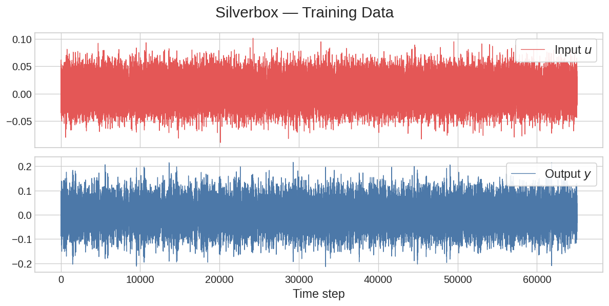
We use the Silverbox benchmark — a standard SISO nonlinear sysid benchmark modelling an electronic circuit that behaves like a Duffing oscillator.
What you will learn:
- How to build a NARX regression dataset with
build_lagged_data - How to use
BSplineFeaturefor smooth nonlinear feature maps - How to train a
TTKMmodel with ALS - How to run closed-loop recursive simulation with
simulate_recursive
from functools import partial

import jax
import numpy as np
import jax.numpy as jnp
import matplotlib as mpl
import matplotlib.pyplot as plt
import nonlinear_benchmarks as nb
from sklearn.preprocessing import MinMaxScaler

from tnkm.models import TTKM
from tnkm.optim import train_als
from tnkm.simulation import simulate_recursive
from tnkm.features import ProductFeatures, BSplineFeature
from tnkm.preprocessing import build_lagged_data, build_lagged_feature

jax.config.update("jax_enable_x64", True)
plt.style.use("seaborn-v0_8-whitegrid")

RC_PARAMS = {
    'figure.facecolor': 'white',
    'font.size': 10,
    'axes.labelsize': 14,
    'axes.grid': True,
    'lines.linestyle': '-',
    'legend.fontsize': 14,
    'xtick.labelsize': 12,
    'ytick.labelsize': 12,
    'axes.titlesize': 16,
    'figure.max_open_warning': 50,
    "legend.frameon": True,
    "legend.framealpha": 0.9,
}

COLORS = dict(
    blue2="#4C78A8",
    red2="#E45756",
    green2="#71b553",
    purple2="#af4d7d"
)
Load & Explore Data
The Silverbox is a SISO benchmark with one training record and three test records. We use the first test record for evaluation.
Note
Unlike the ML examples, we do not shuffle the data. The temporal ordering of samples is essential for time-series models.
(u_train, y_train), test_sets = nb.Silverbox()
test = test_sets[0]
u_train = jnp.array(u_train)
y_train = jnp.array(y_train)
u_test = jnp.array(test.u)
y_test = jnp.array(test.y)
init_len = test.state_initialization_window_length

print(f"Train: {len(u_train)} samples")
print(f"Test: {len(u_test)} samples | warm-up: {init_len} samples")

with mpl.rc_context(RC_PARAMS):
    fig, axes = plt.subplots(2, 1, figsize=(10, 5), sharex=True)
    axes[0].plot(u_train, color=COLORS['red2'],  lw=0.8, label="Input $u$")
    axes[1].plot(y_train, color=COLORS['blue2'], lw=0.8, label="Output $y$")
    for ax in axes:
        ax.legend()
    axes[1].set_xlabel("Time step")
    plt.suptitle("Silverbox — Training Data", fontsize=18)
    plt.tight_layout()
    plt.show()
Train: 65062 samples
Test: 21688 samples | warm-up: 50 samples
Build NARX Feature Matrix
A NARX model predicts the current output from past outputs and past inputs:
build_lagged_data(u, y, input_lags, output_lags) constructs the supervised
dataset. Passing both output_lags and input_lags includes past outputs in
the feature matrix — this gives the model its autoregressive (AR) character.
Note
BSplineFeature maps each input dimension to a B-spline basis defined on
[0, 1]. We therefore scale the entire feature matrix to [0, 1] with
MinMaxScaler fitted on training data only.
input_lags = (0, 1, 2, 3, 4) # u[t], u[t-1], ..., u[t-4]
output_lags = (1, 2, 3, 4) # y[t-1], ..., y[t-4]
d_dim = len(input_lags) + len(output_lags) # 9 lag dimensions

# Lagged regression datasets (original scale)
X_tr, y_tr = build_lagged_data(u_train, y_train, input_lags, output_lags)
X_te, y_te = build_lagged_data(u_test,  y_test,  input_lags, output_lags)

# Scale features to [0, 1] — required by BSplineFeature
x_scaler = MinMaxScaler()
X_tr_sc = jnp.array(x_scaler.fit_transform(np.array(X_tr)))
X_te_sc = jnp.array(x_scaler.transform(np.array(X_te)))

# Scale targets to [0, 1] for training
y_scaler = MinMaxScaler()
y_tr_sc = jnp.array(
    y_scaler.fit_transform(np.array(y_tr)[:, None]).squeeze()
)

print(f"Feature matrix: {X_tr_sc.shape} ({d_dim} lag dimensions)")
print(f"Targets: {y_tr_sc.shape}")
Feature matrix: (65058, 9) (9 lag dimensions)
Targets: (65058,)
Build & Train TTKM
Each lag dimension gets its own BSplineFeature — a piecewise polynomial
basis of order k_order with n_knots equally spaced knot intervals on [0, 1].
The k_col=i argument tells each feature to read column i from the input matrix.
| Parameter | Role |
|---|---|
k_order |
Polynomial order of the B-spline (3 = cubic) |
n_knots |
Number of knot intervals; output dim per lag = n_knots + k_order |
rank |
TT rank — controls model capacity |
ProductFeatures accepts a list of per-dimension feature maps and infers
d_dim automatically from the list length.
ALS updates one TT core at a time while keeping the others fixed.
gamma_w controls L2 regularization.
k_order = 3 # cubic B-splines
n_knots = 6 # knot intervals per dimension
rank = 4 # TT rank

features = ProductFeatures(
    [BSplineFeature(k_order, n_knots, k_col=i) for i in range(d_dim)]
)
model = TTKM(features, rank=rank, seed=0)

train_als(
    model,
    X_tr_sc,
    y_tr_sc,
    n_epoch=10,
    gamma_w=5e-4,
    reg_mode='tensor',
)

# One-step-ahead RMSE on training set
y_tr_pred_sc = model.predict(X_tr_sc)
y_tr_pred = y_scaler.inverse_transform(
    np.array(y_tr_pred_sc)[:, None]).squeeze()
rmse_tr = np.sqrt(np.mean((np.array(y_tr) - y_tr_pred) ** 2))
print(f"Train RMSE (one-step): {rmse_tr:.5f}")
Train RMSE (one-step): 0.00922
One-step-ahead Prediction
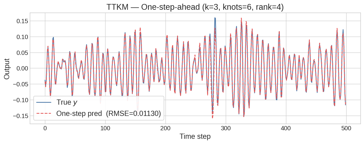
In one-step-ahead prediction the model uses true past outputs at every step — the NARX loop is open. This tests whether the model has learned the input-output mapping before we close the loop.
y_te_pred_sc = model.predict(X_te_sc)
y_te_pred = y_scaler.inverse_transform(
    np.array(y_te_pred_sc)[:, None]).squeeze()
rmse_osa = np.sqrt(np.mean((np.array(y_te) - y_te_pred) ** 2))
print(f"Test RMSE (one-step): {rmse_osa:.5f}")

n_show = 500
with mpl.rc_context(RC_PARAMS):
    fig, ax = plt.subplots(figsize=(10, 4))
    ax.plot(
        np.array(y_te)[:n_show], color=COLORS['blue2'], lw=1.5, label="True $y$"
    )
    ax.plot(
        y_te_pred[:n_show], color=COLORS['red2'], lw=1.5, linestyle="--",
        label=f"One-step pred  (RMSE={rmse_osa:.5f})"
    )
    ax.set_xlabel("Time step")
    ax.set_ylabel("Output")
    ax.set_title(
        f"TTKM — One-step-ahead (k={k_order}, knots={n_knots}, rank={rank})"
    )
    ax.legend()
    plt.tight_layout()
    plt.show()
Test RMSE (one-step): 0.01130
Recursive Simulation
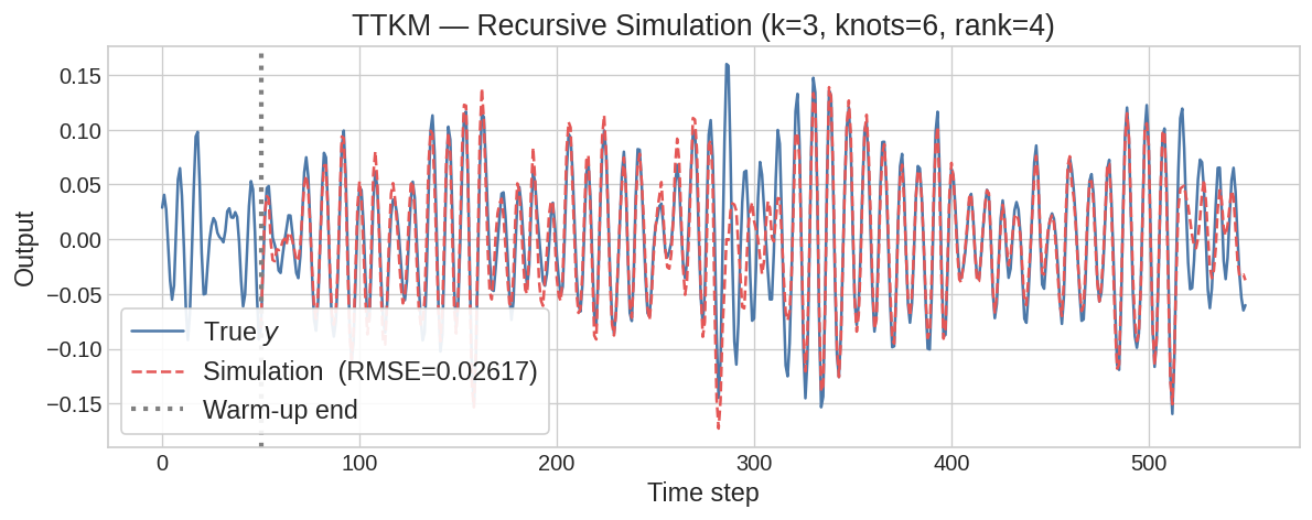
In recursive simulation the model uses its own predictions as past outputs —
the NARX loop is closed. The warm-up window (init_len samples) provides true
initial outputs to bootstrap the recursion; RMSE is measured only on the
remaining steps.
simulate_recursive handles the closed-loop rollout. It expects scalers that
accept and return JAX arrays, so we wrap the scikit-learn MinMaxScaler objects:
class _Scaler:
    """Wrap a scikit-learn scaler to accept and return JAX arrays."""
    def __init__(self, sk_scaler):
        self._sc = sk_scaler
    def transform(self, x):
        return jnp.array(self._sc.transform(np.array(x)))
    def inverse_transform(self, y):
        return jnp.array(self._sc.inverse_transform(np.array(y)))


feature_builder = partial(
    build_lagged_feature,
    input_lags=input_lags,
    output_lags=output_lags,
)

y_sim = simulate_recursive(
    model,
    u_input=u_test,
    y_init_output=y_test[:init_len],
    feature_builder=feature_builder,
    x_sc=_Scaler(x_scaler),
    y_sc=_Scaler(y_scaler),
)

rmse_sim = np.sqrt(np.mean(
    (np.array(y_test[init_len:]) - np.array(y_sim[init_len:])) ** 2
))
print(f"Test RMSE (simulation): {rmse_sim:.5f}")

n_show = 500
with mpl.rc_context(RC_PARAMS):
    fig, ax = plt.subplots(figsize=(10, 4))
    ax.plot(
        np.array(y_test)[:n_show + init_len],
        color=COLORS['blue2'], lw=1.5, label="True $y$"
    )
    ax.plot(
        np.arange(init_len, len(y_test))[:n_show],
        np.array(y_sim[init_len:])[:n_show],
        color=COLORS['red2'], lw=1.5, linestyle="--",
        label=f"Simulation  (RMSE={rmse_sim:.5f})",
    )
    ax.axvline(init_len, color="gray", linestyle=":", lw=2.5, label="Warm-up end")
    ax.set_xlabel("Time step")
    ax.set_ylabel("Output")
    ax.set_title(
        f"TTKM — Recursive Simulation (k={k_order}, knots={n_knots}, rank={rank})"
    )
    ax.legend()
    plt.tight_layout()
    plt.show()
Test RMSE (simulation): 0.02617
Next Steps
- Tune lags: experiment with
input_lagsandoutput_lags— e.g. add longer lags(8, 16, 32)to capture slower system dynamics - Increase B-spline complexity: raise
n_knotsork_orderfor a more expressive per-dimension basis - Switch to CPKM: replace
TTKMwithCPKMfor CP-decomposition-based compression instead of Tensor Train - Use gradient training: replace
train_alswithtrain_grad(e.g. Adam optimizer via Optax) for stochastic mini-batch training