Polynomial Regression on Concrete Compressive Strength
This example shows how to use CPKM (CP Tensor-Network Kernel Machine) with polynomial features for multi-dimensional regression.
We use the Concrete Compressive Strength dataset (UCI) — 8 continuous inputs describing concrete composition, 1030 samples, target is compressive strength in MPa.
What you will learn:
- How to build a
ProductFeaturesmap with per-dimensionPolyFeature - How to train a
CPKMmodel with ALS - How
rankandm_orderaffect model capacity and generalization
import jax
import numpy as np
import jax.numpy as jnp
import matplotlib as mpl
import matplotlib.pyplot as plt
from ucimlrepo import fetch_ucirepo

from tnkm.models import CPKM
from tnkm.optim import train_als
from tnkm.features import ProductFeatures, PolyFeature

jax.config.update("jax_enable_x64", True)
plt.style.use("seaborn-v0_8-whitegrid")

RC_PARAMS = {
    'figure.facecolor': 'white',
    'font.size': 10,
    'axes.labelsize': 14,
    'axes.grid': True,
    'lines.linestyle': '-',
    'legend.fontsize': 14,
    'xtick.labelsize': 12,
    'ytick.labelsize': 12,
    'axes.titlesize': 16,
    'figure.max_open_warning': 50,
    "legend.frameon": True,
    "legend.framealpha": 0.9,
}

COLORS = dict(
    blue2="#4C78A8",
    red2="#E45756",
    green2="#71b553",
    purple2="#af4d7d"
)
Load & Preprocess
The dataset has 8 features (cement, water, slag, etc.) and ~1030 samples.
We apply:
- 80/20 train/test split with a fixed random seed for reproducibility
- Min-max normalization of inputs to \([0, 1]\) using training statistics — this is important for polynomial features, which grow rapidly outside \([0, 1]\)
- Standardization of the output (zero mean, unit variance) to make regularization scale-invariant
Note
All statistics are computed on the training set only to avoid data leakage.
concrete = fetch_ucirepo(id=165)
X_raw = concrete.data.features.to_numpy().astype(float)
y_raw = concrete.data.targets.to_numpy().squeeze().astype(float)

d_dim = X_raw.shape[1]

# 80/20 split
rng = np.random.default_rng(42)
idx = rng.permutation(len(X_raw))
n_train = int(0.8 * len(X_raw))
tr, te = idx[:n_train], idx[n_train:]
X_tr, X_te = X_raw[tr], X_raw[te]
y_tr, y_te = y_raw[tr], y_raw[te]

# Normalize inputs to [0, 1] using training statistics
eps = 1e-8
x_min, x_max = X_tr.min(0), X_tr.max(0)
X_tr = (X_tr - x_min) / (x_max - x_min + eps)
X_te = (X_te - x_min) / (x_max - x_min + eps)

# Standardize output using training statistics
y_mean, y_std = y_tr.mean(), y_tr.std()
y_tr = (y_tr - y_mean) / (y_std + eps)
y_te = (y_te - y_mean) / (y_std + eps)

x_train, y_train, x_test, y_test = map(
    jnp.array, [X_tr, y_tr, X_te, y_te]
)

print(f"Train: {x_train.shape}, Test: {x_test.shape}, d_dim={d_dim}")
Train: (824, 8), Test: (206, 8), d_dim=8
Build & Train CPKM
A CPKM model is defined by:
ProductFeatures— a per-dimension feature map. Here each dimension getsPolyFeature(m_order, k_col=i), producing a feature vector \([1, x_i, x_i^2, \ldots, x_i^{m-1}]\) of lengthm_orderfor each input \(x_i\).rank— the CP rank, controlling the number of rank-1 tensor components. Higher rank → more expressive model.
Training uses Alternating Least Squares (ALS): each tensor core is updated
by solving a regularized least-squares problem while the others are held fixed.
gamma_w controls L2 regularization strength.
m_order = 5 # polynomial order per dimension
rank = 8 # CP rank

features = ProductFeatures(
    [PolyFeature(m_order, k_col=i) for i in range(d_dim)]
)
model = CPKM(features, rank=rank, seed=0)

train_als(model, x_train, y_train, n_epoch=20, gamma_w=1e-4, beta_e=1.0)

y_train_pred = model.predict(x_train)
y_test_pred  = model.predict(x_test)

train_mse = float(jnp.mean((y_train_pred - y_train) ** 2))
test_mse = float(jnp.mean((y_test_pred  - y_test)  ** 2))
print(f"Train MSE: {train_mse:.4f}")
print(f"Test MSE: {test_mse:.4f}")
Train MSE: 0.0490
Test MSE: 0.1217
Results
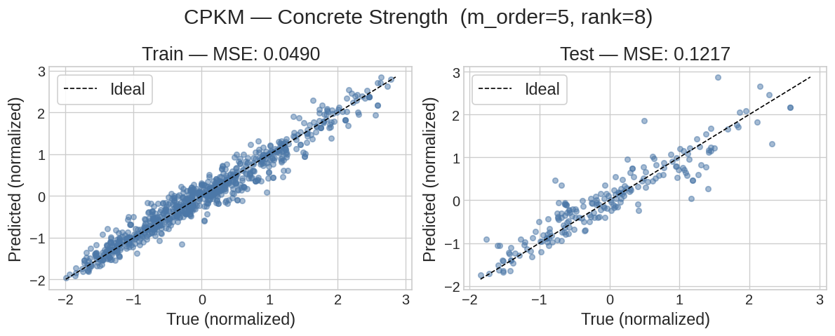
The scatter plots show how well the model generalizes. Points close to the
dashed diagonal indicate accurate predictions. A large gap between train and
test MSE signals overfitting — try increasing gamma_w or reducing rank.
With m_order=5 and rank=8, the model achieves competitive results despite
the full polynomial feature space having \(5^8 = 390{,}625\) entries — the CP
decomposition compresses this to \(8 \times 8 \times 5 = 320\) parameters.
with mpl.rc_context(RC_PARAMS):
    fig, axes = plt.subplots(1, 2, figsize=(10, 4))
    for ax, (y_true, y_pred, split) in zip(
        axes,
        [(y_train, y_train_pred, "Train"), (y_test, y_test_pred, "Test")],
    ):
        lo = min(float(y_true.min()), float(y_pred.min()))
        hi = max(float(y_true.max()), float(y_pred.max()))
        mse = float(jnp.mean((y_pred - y_true) ** 2))
        ax.scatter(y_true, y_pred, s=20, alpha=0.5, color=COLORS['blue2'])
        ax.plot([lo, hi], [lo, hi], "k--", lw=1, label="Ideal")
        ax.set_xlabel("True (normalized)")
        ax.set_ylabel("Predicted (normalized)")
        ax.set_title(f"{split} — MSE: {mse:.4f}")
        ax.legend()

    plt.suptitle(
        f"CPKM — Concrete Strength  (m_order={m_order}, rank={rank})",
        fontsize=18,
    )
    plt.tight_layout()
    plt.show()
Hyperparameter Study
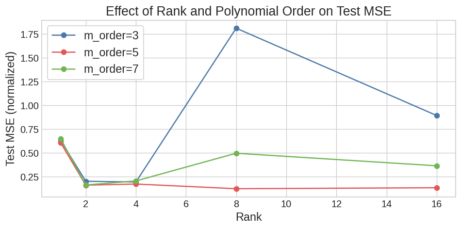
We sweep rank ∈ {1, 2, 4, 8, 16} and m_order ∈ {3, 5, 7} while keeping
all other settings fixed. This illustrates two complementary sources of model
capacity:
| Hyperparameter | Effect |
|---|---|
rank |
Number of rank-1 components; controls global expressiveness |
m_order |
Polynomial degree per dimension; controls local feature resolution |
Higher values of both generally reduce training error, but can overfit.
ranks = [1, 2, 4, 8, 16]
m_orders = [3, 5, 7]

results = {}
for m in m_orders:
    for r in ranks:
        feats = ProductFeatures([PolyFeature(m, k_col=i) for i in range(d_dim)])
        mdl   = CPKM(feats, rank=r, seed=0)
        train_als(mdl, x_train, y_train, n_epoch=20, gamma_w=1e-4, beta_e=1.0)
        y_pred = mdl.predict(x_test)
        results[(m, r)] = float(jnp.mean((y_pred - y_test) ** 2))

color_keys = ["blue2", "red2", "green2"]
with mpl.rc_context(RC_PARAMS):
    fig, ax = plt.subplots(figsize=(8, 4))
    for m, c_key in zip(m_orders, color_keys):
        ax.plot(
            ranks,
            [results[(m, r)] for r in ranks],
            marker="o",
            color=COLORS[c_key],
            label=f"m_order={m}",
        )

    ax.set_xlabel("Rank")
    ax.set_ylabel("Test MSE (normalized)")
    ax.set_title("Effect of Rank and Polynomial Order on Test MSE")
    ax.legend()
    plt.tight_layout()
    plt.show()
Next Steps
- Try TTKM: replace
CPKMwithTTKMto explore an alternative tensor-network parameterization - Experiment with feature maps: replace
PolyFeaturewithFourierFeatureorBSplineFeaturefor different inductive biases - Tune regularization:
gamma_wandbeta_eboth affect bias-variance trade-off; a grid search similar to the one above works well - Use gradient-based optimization: train the same model with
train_gradand compare its convergence behavior and final accuracy with ALS